This blog will represent exploratory data analysis (EDA) of COVID-19 global data and the time series prediction process. The COVID-19 global data is from Kaggle and it contains several key variables such as date, countries, counties, numbers of confirmed cases, and fatalities.

EDA:
Based on the line charts below, we can see that most countries have almost zero records with confirmed cases and fatalities before March 2020. There is a small peak around Feb-15-2020 because COVID-19 happened early in China from December 2019 and the number of confirmed cases reached a peak on Feb-15–2020.
After March 1st, COVID-19 began to ‘eat’ into other countries such as the United States, Korea, Brazil, and Russia. From March 15th, the number of global confirmed cases dramatically increased from 20,000 to 160,000 and after it reached the peak, the number of confirmed cases has kept stationary with some fluctuations between 120,000 to 160,000. Based on the data from different continents, the trend of confirmed cases in Oceania and Europe are similar. Both of them increased to the top and decreased significantly again. Other continents’ numbers of the confirmed cases are still increasing.


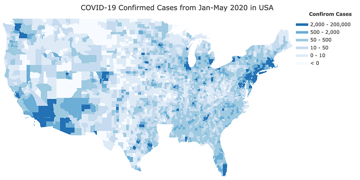
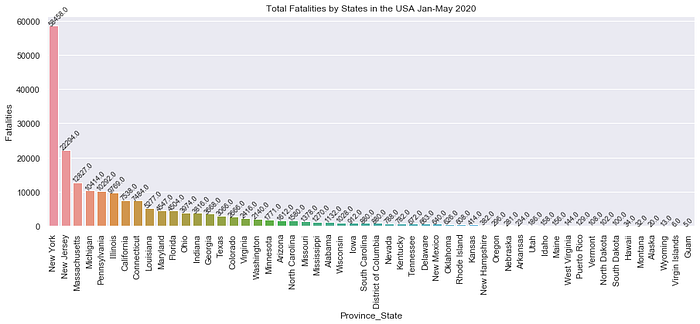
According to the graph of the top 10 countries by confirmed cases and fatalities, both confirmed cases and fatalities rarely happen after March 2020 in China. To help quell its outbreak, the Chinese government put forth strategies to ease the spread of COVID-19. The Chinese government closed all schools, required millions of people to remain indoors, built more than a dozen temporary hospitals, deployed thousands of extra medical staff to Wuhan, and meticulously tested and traced anyone and everyone who may have encountered the virus. On the other hand, the USA has been facing a more serious situation. As of March 2020, the trend of confirmed cases is increasing significantly and more than 300,000 individuals have died because of COVID-19. The confirmed case density map shows that New York, New Jersey, and Massachusetts are near each other, so those three states are the most affected. Michigan, Pennsylvania, Illinois, and Califonia also present high numbers of confirmed cases and based on the bar chart, those states also have high numbers of fatalities. New York has been hit the worst. As of June 1st, 2020, there are 204,000 confirmed cases and 16,410 total deaths.
Data Engineering
Before we apply LSTM, we need to clean our data and do some feature engineering and data pre-processing. Time series data is different from regular numerical data such as housing price data. The time-series data will change by the time and also be affected by other variables, so we cannot simply use mean, median, or mode to fill out the missing data. Two ways can fill out the missing data: one is the forward fill method and one is the backward fill method. If you do not have any missing data then you can simply skip this part!
# Backward Fill method
#(when missing data is located at the begining of the data)
def Backward_Fill(data,col):
    return data[col].bfill()# Fill out the data column by column
#using loop to fill the missing data
for col in data.columns:
    data[col]=Backward_Fill(data,col)
=============================================================
# Forward Fill method
#(when missing data is located at the end of the data)
def Forward_Fill(data,col):
    return data[col].ffill()# Fill out the data column by column
#using loop to fill the missing data
for col in data.columns:
    data[col]=Forward_Fill(data,col)#source:https://www.machinelearningplus.com/time-series/time-series-analysis-python/
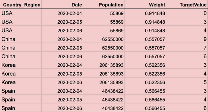
An example is the following: we can see there are four different countries and the date of the data for each country is from Feb 4th to Feb 6th of 2020. If we want to use the forward or backward fill method for panel data, we need to fill out missing values for each column of each country’s data. We can loop each country and loop each column of each country’s data.
#  using loop to fill the missing data
# obtain unique countries
unique_countries=list(set(data.Country_Region))for country in unique_countries:
    df=data[data.Country_Region==country]
    for col in df:
        df[col]=Backward_Fill(df,col)
This part of ‘Train Test Split’ is the trickiest one. The problem is how to correctly split train and test data for time series panel data. We cannot randomly split time series data into 80% and 20% for our train and test data. For example, if we only have one country’s data, then we can split train_data and test_data as follows:
train_data=data.iloc[:int(len(data)*0.8)]
test_data=data.iloc[int(len(data)*0.8):]
The ‘train test split’ for panel data is just split for each country first and we can combine each country's train_data as final train data and also combine each country’s test_data as final test data. Then, we need to reshape our data for our LSTM model. (For more information, please visit my GitHub)
def train_test_split(data):
    size=int(len(data)*0.8)
    # for train data will be collected from each country's data which index is from 0-size (80%)
    x_train =data.drop(columns=['TargetValue']).iloc[0:size]
    # for test data will be collected from each country's  data which index is from size to the end (20%)
    x_test = data.drop(columns=['TargetValue']).iloc[size:]
    y_train=data['TargetValue'].iloc[0:size]
    y_test=data['TargetValue'].iloc[size:]
    return x_train, x_test,y_train,y_test# unique countries
country=list(set(data.country))
# loop each country_Region and split the data into train and test dataX_train=[]
X_test=[]
Y_train=[]
Y_test=[]
for i in range(0,len(country)):
    df=data[['country']==country[i]]    # applied the function I created above
    x_train, x_test,y_train,y_test=train_test_split(df)
    X_train.append(x_train)
    X_test.append(x_test)
    Y_train.append(y_train)
    Y_test.append(y_test)# concatenate each train data n X_train list and Y_train list respectivelyX_train=pd.concat(X_train)
Y_train=pd.DataFrame(pd.concat(Y_train))# concatenate each test dataset in X_test list and Y_test list respectivelyX_test=pd.concat(X_test)
Y_test=pd.DataFrame(pd.concat(Y_test))
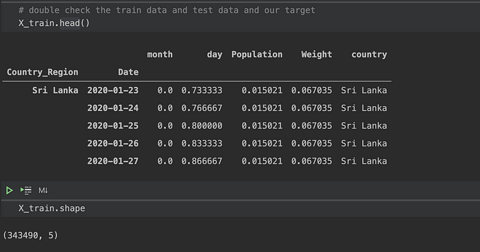
Let us take look at our data! the Country_Region and Date become indexes.
Data Preprocessing
Since want to use today’s data to forecast tomorrow, then we need to do “Lag timestamp”. Thanks Jason Brownlee for sharing this code. For more information, please visit here! The function below is to convert series to supervised learning.
def series_to_supervised(data, n_in=1, n_out=1, dropnan=True):
    n_vars = 1 if type(data) is list else data.shape[1]
    df = DataFrame(data)
    cols, names = list(), list()
    # input sequence (t-n, ... t-1)
    for i in range(n_in, 0, -1):
        cols.append(df.shift(i))
        names += [('var%d(t-%d)' % (j+1, i)) for j in range(n_vars)]
    # forecast sequence (t, t+1, ... t+n)
    for i in range(0, n_out):
        cols.append(df.shift(-i))
        if i == 0:
            names += [('var%d(t)' % (j+1)) for j in range(n_vars)]
        else:
            names += [('var%d(t+%d)' % (j+1, i)) for j in range(n_vars)]
    # put it all together
    agg = concat(cols, axis=1)
    agg.columns = names
    # drop rows with NaN values
    if dropnan:
        agg.dropna(inplace=True)
    return agg
Because we want to use yesterday’s(t-1) data to predict today(t). This is called the lag time. This is the time between two-time series you are correlating. It can be decided with autocorrelation. If you are interested in lag and autocorrelation please visit here!
# an example var1(t-1)  var2(t-1)  var3(t-1)  var4(t-1) target(t-1) target(t)
0.8        0.06       0.5        0.98        1            1
0.75       0.03       0.7        0.85        1            1
...
Finally, the inputs are reshaped into the 3D format - [samples, timesteps, features] and this format is expected by LSTMs.
def reshape_data(train,test):
    #Frame as supervised learning and drop all time t columns except
    reframed_train = series_to_supervised(train, 1, 1)
    reframed_test = series_to_supervised(test, 1, 1)
    # split into train and test sets
    train= reframed_train.values
    test=reframed_test.values
    # split into input and outputs
    train_X, y_train = train[:, :-1], train[:, -1]
    test_X, y_test = test[:, :-1], test[:, -1]
    # reshape input to be 3D [samples, timesteps, features]
    x_train = train_X.reshape((train_X.shape[0], 1, train_X.shape[1]))
    x_test = test_X.reshape((test_X.shape[0], 1, test_X.shape[1]))
    return x_train,x_test,y_train,y_test
Let us use those two functions to get our data ready for LSTM.
encoder = LabelEncoder()
#combine X train and Y train as train data
train_data=pd.DataFrame()
train_data[X_train.columns]=X_train
train_data[Y_train.columns]=Y_train
train_data['country']= encoder.fit_transform(train_data['country'])#combine X test and Y test as test data
test_data=pd.DataFrame()
test_data[X_test.columns]=X_test
test_data[Y_test.columns]=Y_test
test_data['country']= encoder.fit_transform(test_data['country'])# using the function to obtian reshaped data
x_train,x_test,y_train,y_test=reshape_data(train_data,test_data)#take a look at the reshaped data!
x_train
>>>
array([[[0.00000000e+00, 7.33333333e-01, 9.27579992e-03, ...,
         9.27579992e-03, 7.69310930e-02, 7.10000000e+01]],

       [[0.00000000e+00, 7.66666667e-01, 9.27579992e-03, ...,
         9.27579992e-03, 7.69310930e-02, 7.10000000e+01]],
LSTM
Long Short-Term Memory (LSTM) recurrent neural networks are a great algorithm for time series data that can easily adapt to multivariate or multiple input forecasting problems. There are two ways to solve time-series panel data: either loop throughout the model for each country’s data or the countries’ panel data once. If you try both and obtain the RMSE for each way, you can compare the result and choose the best way for your time series panel data.
# design network for confirmed cases data
model = Sequential()
model.add(LSTM(60, activation='relu',input_shape=(x_train.shape[1], x_train.shape[2])))

model.add(Dense(1))
model.compile(loss='mae', optimizer='adam')
# fit network
history = model.fit(x_train, y_train, epochs=30, batch_size=50,  verbose=1, shuffle=False)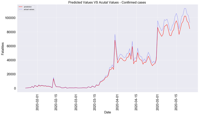
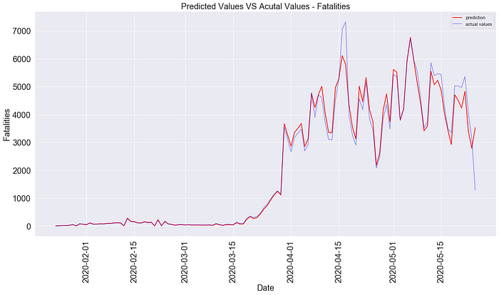
The plot shows the predicted values versus actual values. Our model predicted very well and maybe a little overfitted and the RMSE is around 66 and 17 for confirmed cases and fatalities respectively which are also pretty good results.
Conclusion:
There are different algorithms to deal with time-series data but rarely have very good models for time series panel data. Even though there are statistical models such as Random Effect, Fixed Effect, and pooled OLS models, those models are based on linear models and linear methods can be difficult to adapt to multivariate or multiple input forecasting problems. On the other hand, LSTM is the ideal algorithm for multiple-input forecasting problems and it shows excellent ability to time series panel data forecasting.